Laser-Ion Acceleration

1. From energy density to temperature and pressure

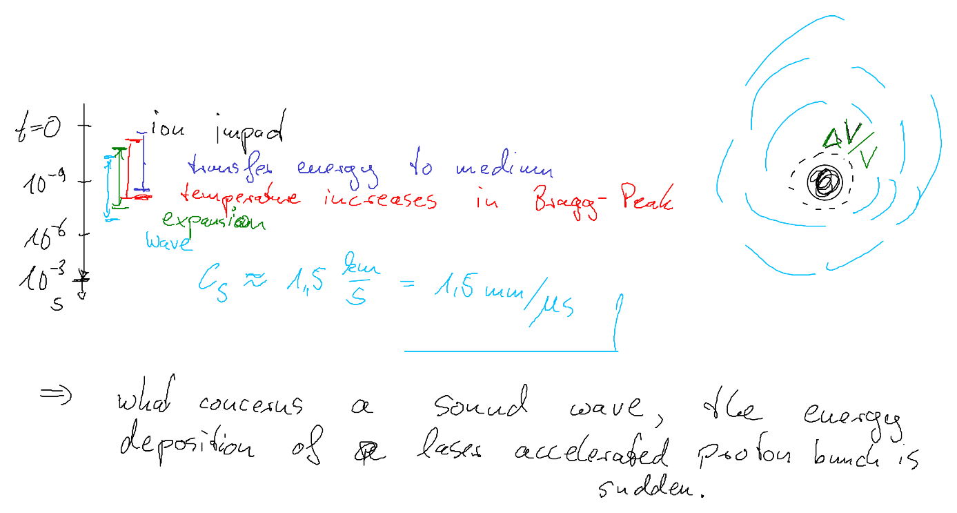
Let \(\varepsilon(\mathbf{r},t)\) be the deposited energy density. If deposition is fast compared with mechanical expansion (stress confinement) and heat diffusion (heat confinement), the heated volume has not yet moved or cooled: temperature rises at constant volume, \[ \Delta T(\mathbf{r}) \approx \frac{\varepsilon(\mathbf{r})}{\rho\,c_V}. \] Stress confinement for a feature of size \(a\) and sound speed \(c_s\) requires \(t_{\mathrm{dep}}\ll a/c_s\) (for water \(c_s\approx 1.5\,\mathrm{mm/\mu s}\)). Heat confinement is far weaker (thermal diffusion times of order seconds for millimetre scales). Laser-driven and many conventional bunches easily satisfy both for MHz acoustics.

2. Thermoacoustic wave equation

Linearised fluid equations plus thermal expansion yield the thermoacoustic wave equation. One common form is \[ \left(\nabla^2 - \frac{1}{c_s^2}\partial_t^2\right)p = -\frac{\beta}{c_p}\,\partial_t^2 \varepsilon = -\frac{\Gamma}{c_s^2}\,\partial_t H, \] where \(\beta\) is the volume thermal expansion coefficient, \(c_p\) the specific heat, \(\Gamma=\beta c_s^2/c_p\) the (dimensionless) Grüneisen parameter, and \(H=\partial_t\varepsilon\) the heating function. The second time derivative of the temperature (or of \(\varepsilon\)) acts as a source of sound.

Separating \(H(\mathbf{r},t)=\varepsilon(\mathbf{r})\,h(t)\) with \(\int h\,\mathrm{d}t=1\) gives a pressure that is the convolution of a spatial Green’s response with the temporal heating profile \(h(t)\).

3. Ultrashort bunch: far-field acoustic trace

For an essentially instantaneous deposition, \(\varepsilon(\mathbf{r},t)=\varepsilon(\mathbf{r})\,\delta(t)\) (i.e.\ \(H=\varepsilon\,\delta(t)\)), the initial-value problem is \(p(\mathbf{r},0)=\Gamma\varepsilon(\mathbf{r})\), \(\partial_t p=0\), after which \(p\) obeys the homogeneous wave equation. A detector in the far field then records a pressure time trace proportional to the negative directional derivative of the energy density along the line of sight (compression leads), sampled at the distance \(c_s t\) from the detector: \[ p(\mathbf{r}_{\mathrm{det}},t) \;\propto\; -\hat{\mathbf{u}}\cdot\nabla\varepsilon \Big|_{\mathbf{r}_{\mathrm{det}}-\hat{\mathbf{u}}\,c_s t}, \] where \(\hat{\mathbf{u}}\) points from the deposit toward the detector (so the arrival time depends on both source and detector position; geometric \(1/R\) factors omitted — see Exercise 14). For a beam-like deposition along \(z\) with transverse profile \(\Phi_\perp\), the on-axis far-field signal is essentially the (negative) derivative of the (spread-out) Bragg curve — the acoustic trace of I-BEAT.

Entrance-window reflection. Part of the thermoacoustic wave propagates upstream (against the ion beam), toward the water–vacuum (or window) interface at the entrance \(z=0\). That interface is to a good approximation a pressure-release boundary: the acoustic amplitude reflection coefficient is \(r=-1\) (vanishing pressure in vacuum). In the method of images this is an odd extension of the initial pressure across \(z=0\). The reflected wave returns and reaches an axial downstream detector later than the direct Bragg signal; the extra path is essentially twice the penetration depth, so the delay between direct and reflected arrivals measures the Bragg-peak depth \(\Delta t \approx 2 z_{\mathrm{peak}}/c_s\) (for an on-axis geometry). Toggle reflect z=0 in Fig. 14.2 to see the delayed “refl.” feature on the trace.

I-BEAT 3D. A single far-field trace already encodes the depth dose derivative (Fig. 14.2). Adding transducers off axis (top / left / right, …) measures different path lengths from the same Bragg-peak source: the set of arrival times trilaterates the deposit, while relative amplitudes and waveform shapes constrain transverse size and pointing. In practice this yields ion energy, energy spread, spot size, beam position and particle number from one bunch — without an RCF stack (Gerlach et al., HPLSE 11, e38 (2023); class data slides).

4. Outlook

I-BEAT closes the instrumentation arc that began with magnets and RCF: spectrum → depth dose → heat → sound. Lecture 15 summarises the course and open questions (efficiency, repetition rate, beam quality, applications).