- The laser–plasma source is a point-like, divergent, polyenergetic spray. Many applications need a transported, energy-selected beam at an irradiation platform.
- A magnetic quadrupole focuses in one transverse plane and defocuses in the other; a doublet (opposite polarity) focuses both.
- Focusing strength scales with \(1/(B\rho)\propto 1/p\) → strong chromaticity: the doublet is an energy filter. A millimetre aperture at the focus selects \(\Delta E/E\).
- That monoenergetic pencil beam is the prerequisite for a clean Bragg peak and for I-BEAT (Lecture 14).
Lecture 12 closed with monoenergetic heavy ions drawing a Bragg curve in an interferogram. Laser-driven protons start as a spray. To recover a similar local Bragg source we need transport and energy selection — at CALA typically a permanent-magnet quadrupole doublet.
1. Why transport?
Some applications embrace the raw divergent spray (large-field radiography, isochoric heating). Most traditional irradiation studies want a beam: controlled spot, known energy, reduced background. Transport almost always implies charge and energy selection. The price is particle number — only a slice of the spectrum and solid angle survives.
2. Magnetic quadrupole
Assume a design trajectory along \(z\) with small transverse deviations \(x,y\) and angles \(x'=p_x/p_z\), \(y'=p_y/p_z\). Ideal quadrupoles have only transverse fields linear in the coordinates, \[ B_x = g\,y,\qquad B_y = g\,x \] (sign convention depending on polarity), with gradient \(g=\partial B_y/\partial x\). The Lorentz force then yields independent Hill equations \[ x'' + k\,x = 0,\qquad y'' - k\,y = 0 \] (or swapped), where the focusing strength is \[ k = \frac{|q|g}{p} = \frac{g}{B\rho}. \] One plane focuses (\(k>0\)), the other defocuses. Hence a single quadrupole cannot make a round focus — we need at least a doublet.
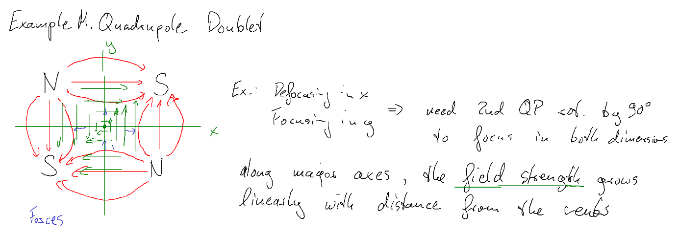
3. Transfer matrices and thin-lens intuition
Solutions of the Hill equations are written as \(2\times 2\) transfer matrices acting on phase-space vectors \((x,x')\) and \((y,y')\). A drift of length \(L\) is \[ M_{\mathrm{d}} = \begin{pmatrix} 1 & L \\ 0 & 1 \end{pmatrix}. \] A focusing quadrupole of length \(\ell\) has trigonometric / hyperbolic entries with argument \(\sqrt{|k|}\,\ell\). In the thin-lens limit \(\ell\to 0\) with \(1/f = |k|\ell\) kept finite, \[ M_{\mathrm{f}} = \begin{pmatrix} 1 & 0 \\ -1/f & 1 \end{pmatrix}. \] A parallel ray at height \(x\) acquires angle \(-x/f\) and crosses the axis after a distance \(f\). A doublet is the product of focusing and defocusing matrices with a short drift between them, followed by a long drift to the application platform (\(\sim 2\,\mathrm{m}\) at CALA-like setups).
4. Chromaticity = energy selection
Because \(k\propto 1/p\), lower-energy protons are over-focused and higher-energy protons under-focused. At a fixed image plane only a narrow energy band lands inside a small aperture. The doublet is therefore both a lens and a spectrometer. Typical permanent-magnet gradients are hundreds of T/m over a few centimetres of iron length (example numbers for Exercise 13: \(g\sim 300\,\mathrm{T/m}\), \(\ell_1\sim 4\,\mathrm{cm}\), \(\ell_2\sim 2\,\mathrm{cm}\)). Drag the quadrupoles in the simulator below, press Focus E₀, then enable Show non-focused energies to see chromatic over-/under-focus. (Open full page.)
Bottom line. After transport we have a reasonably monoenergetic, focused proton bunch — precisely the beam that deposits a sharp Bragg peak and launches a localised acoustic wave (Lecture 14, I-BEAT).
5. Beyond permanent-magnet quadrupoles
Round focusing (both planes at once) needs a different field geometry: solenoids (\(B_z\), Larmor-frame focusing) or active plasma / lithium lenses (\(B_\varphi\propto r\), current through the bore). The companion page Focusing of charged particles develops the common equation \(x''+Kx=0\), the DOFO penalty, chromaticity \(\propto 1/(B\rho)\) vs \(\propto 1/(B\rho)^2\), and an interactive trajectory panel for all three technologies.