This sheet accompanies Lecture 7. Part A estimates the cycle-averaged hot-electron density that feeds the rear-side sheath (context for TNSA). Part B asks you to reproduce in PIC the situation of Figure 7.4 — absorption, hot electrons, charge separation, and sheath fields. Use the browser-based 1D3V PIC simulator for Part B.
Part A — Cycle-averaged hot-electron bunch parameters
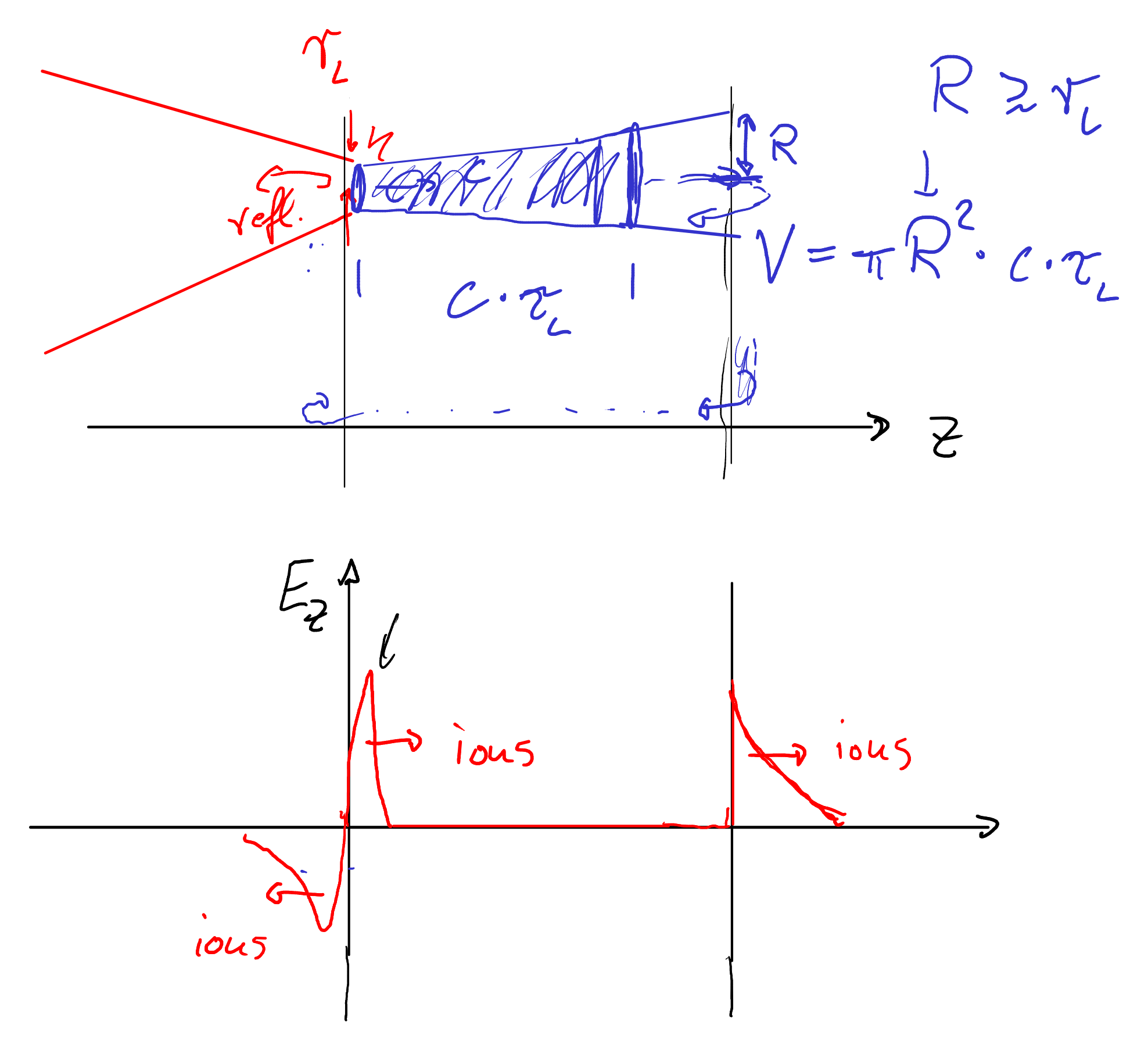
Review Lecture 7, §7 (bridge to ion acceleration). Here \(R\) is the electron-beam radius at the rear side, not the laser focal spot \(r_L\).
-
Hot-electron density.
Assume a laser pulse with energy \(E_L\) and duration \(\tau_L\) irradiates a vacuum–overdense
plasma interface at normal incidence with focal-spot radius \(r_L\). A fraction \(\eta\) of the
laser energy is converted into kinetic energy of forward-going electrons that travel at
\(v_e\approx c\), cross a foil of thickness \(d\), and exit on the rear (non-irradiated) side
spread over a circular area of radius
\[
R = r_L + d\,\tan\theta,
\]
where \(\theta\) is a representative divergence half-angle in the plasma.
- Provide an estimate for the cycle-averaged particle density \(n_{e,0}\) of this hot (relativistic) electron bunch. Express \(N_h\) in terms of \(\eta\), \(E_L\), and a representative electron energy \(E_e\), and show \[ n_{e,0} \approx \frac{N_h}{\pi R^2\, c\,\tau_L} = \frac{\eta E_L}{E_e\,\pi R^2\, c\,\tau_L}. \]
- For sufficiently relativistic lasers, the representative energy is often written \[ E_e \approx m_ec^2\sqrt{\frac{I_L\lambda^2}{I_{0,\lambda^2}}}, \qquad I_{0,\lambda^2} = 1.37\times 10^{18}\,\mathrm{W\,cm^{-2}\,\mu m^{2}}. \] Show that both \(E_e\) and \(n_{e,0}\) then scale as \(\sqrt{I_L\lambda^2}\) (for fixed \(\eta\), \(R\), and \(\lambda\)).
Part B — PIC: from absorption to boundary sheath fields
Useful diagnostics include field energy, particle kinetic energy, phase-space plots, and \(E_z(x)\). In 1D there is no transverse spot size: map the heated slab thickness / pulse length onto the idea of an interaction volume \(\sim\pi R^2 c\tau_L\) conceptually when you write up.
- Setup. Configure an overdense plasma slab (\(n_e \gg n_c\)) irradiated at normal or near-normal incidence with \(a_0 \gtrsim 1\). Include mobile ions (not fixed background). Choose pulse duration and slab thickness so that hot electrons can recirculate and sheaths form at both surfaces during/after the pulse. Document your parameters and justify that the target is overdense and relativistic.
- Reflected vs absorbed energy. During and after the pulse, identify how much laser energy is reflected (field energy leaving the simulation domain) versus absorbed (net increase in total particle kinetic energy). Report approximate fractions and describe how you extracted them from the PIC diagnostics. Relate the absorbed fraction qualitatively to \(\eta\) in Part A.
- Electrons hot, ions cold (during pulse). While the laser is on, show that electrons become energetic and can stream or recirculate, whereas ions remain largely immobile on the pulse time scale. Support with phase-space snapshots or energy-vs-time plots for each species.
- Sheath fields. Locate regions of charge separation and the associated quasi-static longitudinal field \(E_z\) at the front (laser-irradiated) and rear surfaces. Plot or sketch \(E_z(x)\) at a time when the pulse is still on or just after it ends.
- Ion acceleration after the pulse. Continue the simulation (or examine late-time frames) to observe ion acceleration driven by the sheath fields — predominantly from the rear surface (TNSA-like) and/or from the front, depending on your setup. Compare qualitatively with the narrative in Figure 7.4.
- Short write-up. In half a page, explain how your PIC movie maps onto Figure 7.4 and Part A: where energy is absorbed, how hot electrons recirculate, where sheath fields form, and what accelerates the ions. Note any features your 1D run cannot capture compared to the 2D schematic (in particular transverse divergence and \(R\neq r_L\)).