Laser-Ion Acceleration – Lecture 7: Relativistic effects and the PIC approach

1. Relativistic plasma optics: why it matters

At sufficiently high laser intensity, the electron quiver motion becomes relativistic. A convenient measure is the normalized vector potential \(\,a_0 = \frac{eE_0}{m_e c \omega_0}\,\). When \(a_0 \gtrsim 1\), the electron Lorentz factor \(\gamma\) is no longer close to unity, and the plasma response changes qualitatively.

1.1 Relativistic transparency

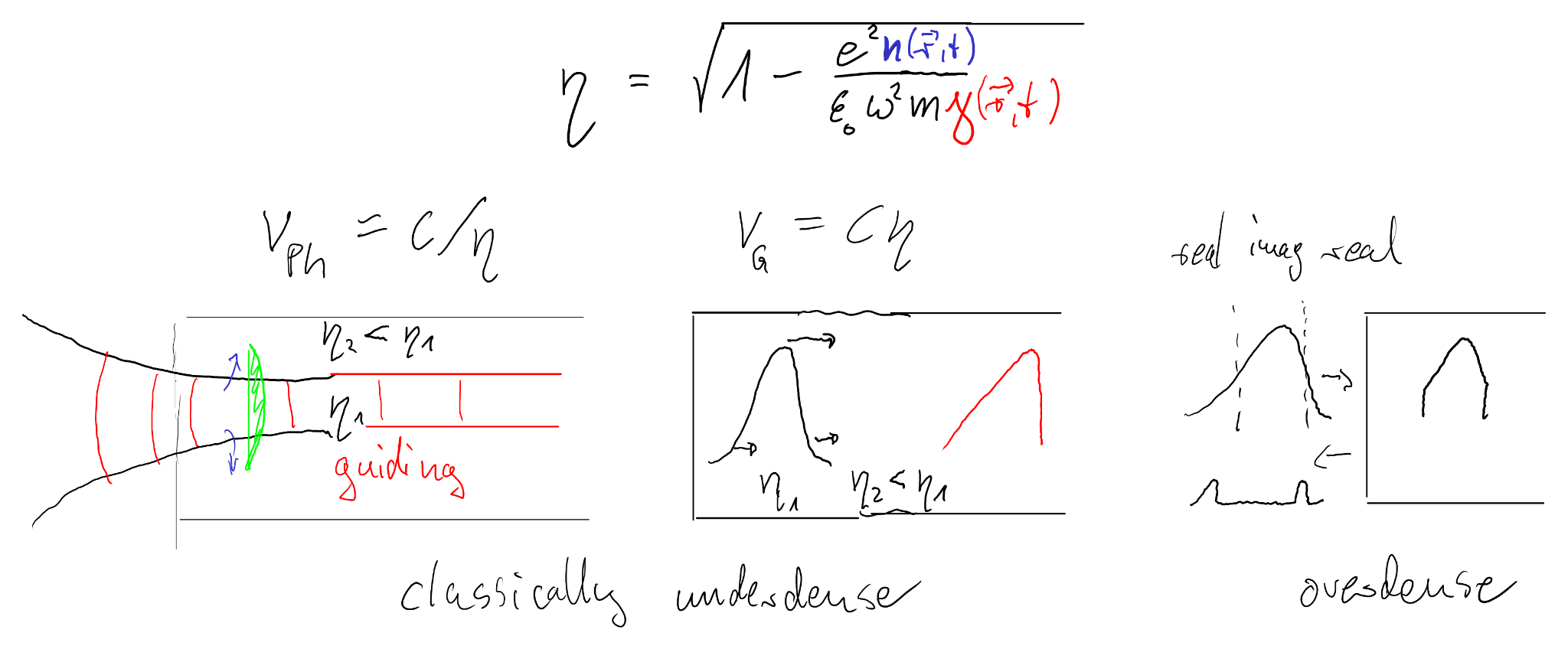
The key idea is that the effective electron mass increases: \(m_e \rightarrow \gamma m_e\). As a result, the plasma frequency decreases, \(\omega_p \propto 1/\sqrt{\gamma}\), and the critical density effectively increases: \[ n_c = \frac{\varepsilon_0 m_e \omega_0^2}{e^2} \quad \Rightarrow \quad n_{c,\mathrm{rel}} \approx \gamma\, n_c. \] An overdense target (\(n_e>n_c\)) can therefore become partially transparent once the electrons are driven relativistically.

1.2 Relativistic self-focusing and channel guiding

In an underdense plasma, the refractive index depends on intensity via \(\gamma(I)\). Higher intensity lowers \(\omega_p\) and increases the local refractive index, so the plasma acts as a focusing medium. This is the basis of relativistic guiding / channeling, and it is one route to long-distance propagation of intense pulses.

1.3 Self-phase modulation

The intensity-dependent refractive index also means the phase velocity varies across the pulse envelope, which broadens the spectrum (self-phase modulation) and can create steepened waveforms.

1.4 “Gate” / inverse to a plasma mirror

A plasma mirror is normally reflective once a solid-density plasma forms at the surface. The inverse concept is a transient “gate”: a target that is reflective at low intensity, but becomes transmissive at high intensity (e.g. by relativistic transparency), enabling temporal or spatial gating of the field.

Relativistic plasma optics: self-focusing/guiding, pulse-front steepening, induced transparency. — **Figure 1:** Relativistic plasma optics (schematic). From left to right: (i) relativistic self-focusing and guiding due to an intensity-dependent refractive index, (ii) pulse-front steepening / self-phase modulation as \(n(\mathbf{r},t)\) varies during the pulse, (iii) relativistic induced transparency (“gate”) when the effective \(\gamma\) reduces \(\omega_p^2/\gamma\) so that a previously overdense layer becomes transparent.

2. The “complete” problem: Maxwell + Vlasov (kinetic)

The full collisionless laser–plasma interaction problem can be written as Maxwell’s equations coupled to a kinetic equation for each species \(s\) (electrons, ions), typically the Vlasov equation. The distribution function \(f_s(\mathbf{x},\mathbf{p},t)\) evolves self-consistently with the fields \(\mathbf{E},\mathbf{B}\).

2.1 Maxwell equations (SI units)

\[ \nabla \cdot \mathbf{E} = \frac{\rho}{\varepsilon_0},\qquad \nabla \cdot \mathbf{B} = 0, \] \[ \nabla \times \mathbf{E} = -\frac{\partial \mathbf{B}}{\partial t},\qquad \nabla \times \mathbf{B} = \mu_0 \mathbf{J} + \mu_0 \varepsilon_0 \frac{\partial \mathbf{E}}{\partial t}. \] Here \(\rho(\mathbf{x},t)=\sum_s q_s \int f_s\, d^3p\) and \(\mathbf{J}(\mathbf{x},t)=\sum_s q_s \int \mathbf{v}\, f_s\, d^3p\).

2.2 Vlasov equation

\[ \frac{\partial f_s}{\partial t} + \mathbf{v}\cdot\nabla_{\mathbf{x}} f_s + q_s \left( \mathbf{E} + \mathbf{v}\times\mathbf{B} \right)\cdot\nabla_{\mathbf{p}} f_s = 0, \] with relativistically consistent \(\mathbf{p}=\gamma m_s \mathbf{v}\), \(\gamma=\sqrt{1+(p/m_sc)^2}\).

Fluid models are obtained by taking velocity moments of the Vlasov equation and adding closure assumptions (equation of state, heat flux, etc.). PIC avoids such closures by evolving representative phase-space samples (“macro-particles”) directly.

3. Particle-in-Cell: the idea, in one page

PIC is a numerical approach to the kinetic-Maxwell system: we represent each species distribution \(f_s\) by a large number of computational particles (“macro-particles”), and we solve Maxwell’s equations on a spatial grid. Currents and charges are obtained by depositing particle contributions onto the grid, and fields are interpolated back to particle positions.

One PIC time step (leapfrog view)

Deposit charge density \(\rho^n\) and/or current \(\mathbf{J}^{n+1/2}\) from particles to the grid (shape functions).
Field solve Maxwell’s equations on the grid to obtain \(\mathbf{E}^{n+1}\), \(\mathbf{B}^{n+1/2}\) (e.g. Yee/FDTD).
Interpolate \(\mathbf{E},\mathbf{B}\) from grid nodes to each particle position.
Push particles using the Lorentz force (commonly the Boris pusher; relativistically correct).
Apply boundary conditions (fields and particles), then repeat.

Why “macro-particles” work (and what they cost)

Each macro-particle represents many physical particles. The method converges as the number of macro-particles per cell increases, but finite particle number introduces statistical noise \(\propto 1/\sqrt{N_p}\). Smoothing, filtering, and careful current deposition can reduce noise without destroying key physics.

4. 1D3V PIC equations (propagation direction is always \(z\))

In this course we use a 1D3V model: one spatial coordinate \(z\), but three velocity (or momentum) components \((v_x,v_y,v_z)\). All field quantities vary only with \(z\) and \(t\), i.e. \(\partial/\partial x=\partial/\partial y = 0\).

4.1 Fields to evolve

A common electromagnetic 1D implementation evolves the transverse fields \((E_x,E_y,B_x,B_y)\) with propagation along \(z\). The longitudinal field \(E_z\) is not obtained by integrating Gauss’ law along \(z\) in time-stepping codes; instead it is updated from the \(z\)-component of Ampère–Maxwell’s law (equivalently, from a charge-conserving scheme that enforces it). Gauss’ law then acts as a constraint (and a useful diagnostic) that is automatically preserved if it holds initially and the discrete continuity equation is satisfied.

4.2 Maxwell in 1D (variation only along \(z\))

With \(\partial_x=\partial_y=0\), curl equations reduce to coupled pairs for the transverse components:

\[ \frac{\partial B_x}{\partial t} = +\frac{\partial E_y}{\partial z}, \qquad \frac{\partial B_y}{\partial t} = -\frac{\partial E_x}{\partial z}, \] \[ \frac{\partial E_x}{\partial t} = -\frac{1}{\varepsilon_0}\, J_x - c^2 \frac{\partial B_y}{\partial z}, \qquad \frac{\partial E_y}{\partial t} = -\frac{1}{\varepsilon_0}\, J_y + c^2 \frac{\partial B_x}{\partial z}. \] The longitudinal electric field is best obtained from the \(z\)-component of Ampère–Maxwell’s law. In 1D (\(\partial_x=\partial_y=0\)) the \(z\)-component of \(\nabla\times\mathbf{B}\) vanishes, so \[ \frac{\partial E_z}{\partial t} = -\frac{1}{\varepsilon_0}\,J_z. \] Gauss’ law, \[ \frac{\partial E_z}{\partial z} = \frac{\rho}{\varepsilon_0}, \] is a constraint (not an evolution equation). It is automatically preserved if it is satisfied initially and if the code respects the continuity equation \[ \frac{\partial \rho}{\partial t} + \frac{\partial J_z}{\partial z} = 0 \] (this is why charge-conserving current deposition matters). In particular, with initially neutral plasma (\(\rho=0\)) and \(E_z=0\), Gauss’ law remains fulfilled up to numerical error.

4.3 Particle equations of motion (3V)

\[ \frac{d\mathbf{p}}{dt} = q\left(\mathbf{E} + \mathbf{v}\times \mathbf{B}\right),\qquad \frac{d\mathbf{x}}{dt} = \mathbf{v} = \frac{\mathbf{p}}{\gamma m}, \] with \(\mathbf{x}=(0,0,z)\) in 1D and \(\mathbf{p}=(p_x,p_y,p_z)\) fully 3D.

Implementation note: why 1D3V still captures “relativistic” physics

The electron dynamics in the laser field is inherently vectorial (transverse quiver, longitudinal drift), which requires 3V. Many effects—relativistic transparency, dispersion, wave excitation, reflection, and even high-harmonic generation (in a reduced sense)— can be explored meaningfully in 1D3V, while keeping the model simple and interactive.

4.4 Normalizations (common in PIC)

Many codes normalize time to \(\omega_0^{-1}\), length to \(k_0^{-1}\) (or \(\lambda_0\)), fields to \(m_ec\omega_0/e\), density to \(n_c\), and momentum to \(m_ec\). If you see dimensionless fields \(a(z,t)\), that is essentially \(a=eA/(m_ec)\).

5. Numerical choices & practical pitfalls

5.1 Grid and time step

Courant condition for FDTD: \(\Delta t \lesssim \Delta z / c\).
Resolve plasma oscillations: \(\Delta t \ll \omega_p^{-1}\) in the densest region you care about.
Resolve Debye length if you want thermal electrostatics; for cold-plasma optics, this is less critical.

5.2 Particle number, noise, and smoothing

Noise decreases as \(1/\sqrt{N_p}\); too few particles per cell can hide subtle physics.
Smoothing helps, but excessive smoothing can suppress real instabilities and high-harmonic content.

5.3 Boundary conditions

Fields: absorbing boundaries (PML) or simple damping layers prevent artificial reflections.
Particles: thermal bath / reflecting / open boundaries, depending on scenario.
Laser injection: boundary-driven transverse fields (e.g. prescribing \(E_x,B_y\) at \(z=0\)).

Interactive follow-up

The concepts in this lecture become much more tangible when you can watch fields, densities, and phase space evolve in time. In Lecture 8, the interactive 1D3V PIC code is used (propagation along \(z\)) as a guided virtual lab: 20251126_pic1d3v_with_CHATGPT.html.