Laser-Ion Acceleration

This sheet accompanies Lecture 10. Part A is the magnetic spectrometer. Part B is Bethe–Bloch and the depth–dose / Bragg curve — the stopping physics behind filters, CR-39 pit size, and the spread-out Bragg peak of Lecture 11.

Part A — Magnetic spectrometer

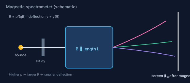
1. Deflection. Consider a point-like source that emits ions with a variety of charge states \(Q\) and mass numbers \(A\), each covering a wide range of momentum \(p\). A slit aperture at distance \(L_1\) with height \(\mathrm{d}y\) collimates the spray and marks the entrance to a permanent-magnet dipole of length \(L\) and field \(B\). The dispersed beam is captured on a screen a distance \(L_2\) after the magnet exit.
   1. Derive a formula for the deflection \(y\) on the screen (magnetic rigidity \(R=p/(qB)\)).
   2. Approximate for small deflection angles (\(L/R\ll 1\)).
2. Spectrum from a line-out. Assume you have already integrated the screen signal along the slit dimension and converted it into a particle fluence map \(\mathrm{d}N/\mathrm{d}y(y)\). Derive an expression for the differential energy distribution \[ \frac{\mathrm{d}^3 N}{\mathrm{d}\Omega\,\mathrm{d}E_k}(E_k). \] Relate \(R\) to kinetic energy \(E_k\) relativistically, \[ p = mc\sqrt{\left(1+\frac{E_k}{mc^2}\right)^2-1}, \] and obtain \(\mathrm{d}y/\mathrm{d}E_k\).
3. Species degeneracy. A proton with kinetic energy \(E_p\) and a fully ionized carbon ion (\(^{12}\mathrm{C}^{6+}\)) land on the same screen position. What is the carbon kinetic energy \(E_C\)? Give the exact (relativistic rigidity) relation and the non-relativistic limit. Comment on why magnetic spectrometry alone cannot identify the ion species, and how filters / Bethe–Bloch (Part B) help.
4. Optional bridge. Sketch how a Thomson parabola (\(E\parallel B\)) would lift the degeneracy of Question 3. No full derivation required — qualitative loci on the detector plane are enough.

Tip (Part A): the non-relativistic carbon–proton relation reduces to equal energy per nucleon times a charge/mass factor — check Lecture 10 §2.

Part B — Bethe–Bloch and depth–dose curve

5. Stopping power vs. energy. Go to NIST PSTAR and extract the total stopping power of protons in water for particle energies from \(0.1\) to \(100\,\mathrm{MeV}\). Plot the energy loss per unit length \(-\mathrm{d}E/\mathrm{d}x\) as a function of \(E_k\).
6. Bethe formula. Add \(-\mathrm{d}E/\mathrm{d}x(E_k)\) as predicted by the Bethe(–Bloch) formula to the same plot. A convenient form (projectile charge number \(z\), electron density \(n\) of the medium, mean excitation energy \(I\)) is \[ -\frac{\mathrm{d}E_{\mathrm{kin}}}{\mathrm{d}\ell} = \frac{4\pi n z^{2}}{\beta^{2}} \left(\frac{e^{2}}{4\pi\varepsilon_{0}}\right)^{2} \frac{1}{m_{e}c^{2}} \Biggl[ \ln\!\left( \frac{2 m_{e}c^{2}\beta^{2}}{I\,(1-\beta^{2})} \right) -\beta^{2} \Biggr], \] with \(\beta=\sqrt{1-1/(1+E_{\mathrm{kin}}/mc^{2})^{2}}\). For water you may use \(I\approx 75\,\mathrm{eV}\) (PSTAR value). Comment on where the formula agrees with PSTAR and where it fails.
7. Depth distribution / Bragg curve. Calculate and plot the depth distribution of deposited energy \(\mathrm{d}E/\mathrm{d}x(x)\) in water for an initial kinetic energy \(E_{k,0}=10\,\mathrm{MeV}\). (Useful approach: integrate the equation of motion with a decelerating force \(-\mathrm{d}E/\mathrm{d}x(E)\), or change variables to obtain \(\beta(x)\) / \(E(x)\) and then evaluate stopping along the path.)
8. Dose. Describe how the depth distribution of deposited energy relates to the depth–dose curve \(D(x)\). Briefly connect this monoenergetic Bragg peak to the spread-out Bragg curve expected from a broad laser–ion spectrum (Lecture 11).

Tip (Part B): keep units consistent (eV vs. J, keV/µm vs. MeV/cm). You may implement the integration in Python or MATLAB.