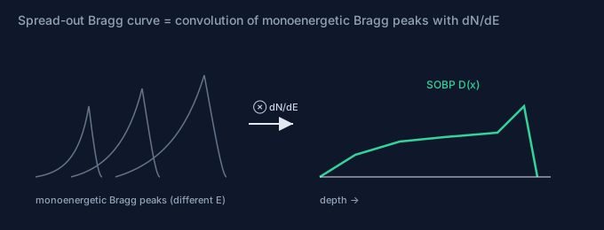
- A polyenergetic spectrum turns monoenergetic Bragg peaks into a spread-out Bragg curve (SOBP) — a convolution (Faltung) of \(-\mathrm{d}E/\mathrm{d}x\) with \(\mathrm{d}N/\mathrm{d}E\).
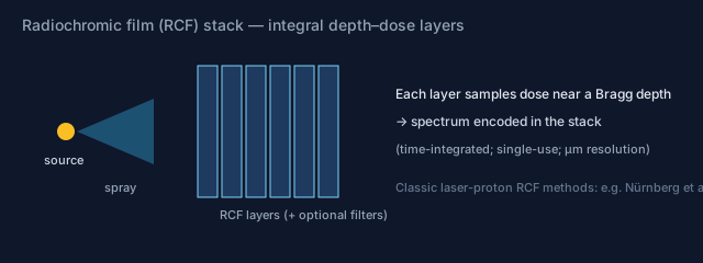
- RCF stacks record that depth dose integrally (µm layers); classic laser-proton imaging spectroscopy is documented e.g. by Nürnberg et al. (2009) — shown in class slides, not reproduced here.
- Clinics build SOBPs over many monoenergetic bunches (minutes); a laser point source with a pinhole yields a polyenergetic pencil beam with locked longitudinal emittance → time-resolved SOBP and TOF spectroscopy.
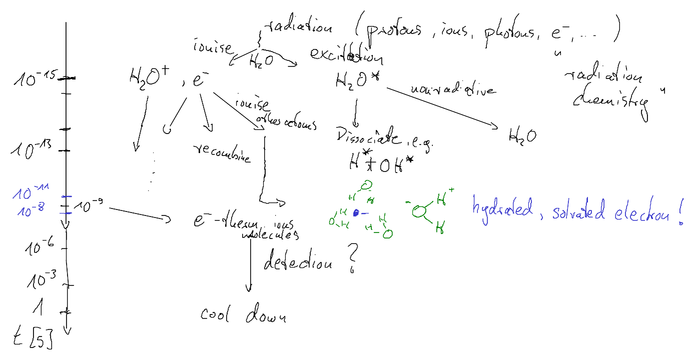
- Deposited energy ionizes water; liberated electrons thermalize and become solvated — optically absorbing, hence probeable with a laser.
Lecture 10 ended with Bethe–Bloch: a monoenergetic ion deposits energy in a Bragg peak. Laser–plasma sources, however, deliver broad spectra. Today we fold those spectra into depth–dose distributions, connect them to radiochromic-film practice, and ask what happens to the deposited energy in water on picosecond–nanosecond scales.
1. Spread-out Bragg curve as a convolution
Let \(b(x;E_0)\) be the depth dose (or \(\mathrm{d}E/\mathrm{d}x\) along the path) of a particle that entered with kinetic energy \(E_0\). For a continuous spectrum \(\mathrm{d}N/\mathrm{d}E\) the observed depth distribution is the superposition \[ D(x) \propto \int \frac{\mathrm{d}N}{\mathrm{d}E}(E)\, b(x;E)\, \mathrm{d}E \] — a convolution / Faltung of Bragg curves with the energy distribution. High-energy components push the distal edge deeper; low-energy components fill the entrance plateau. An approximately exponential laser–proton spectrum therefore produces a broad “spread-out” Bragg curve rather than a single sharp peak.
2. Radiochromic film stacks — and the clinical contrast
A practical integral detector is a radiochromic film (RCF) stack: many thin active layers (often interleaved with filters) darken in proportion to local dose. Because different proton energies stop at different depths, the stack encodes the spectrum in the layer-by-layer dose pattern — radiochromic film imaging spectroscopy. A standard reference for laser-accelerated protons is Nürnberg et al., Rev. Sci. Instrum. 80, 033301 (2009); representative stack images are shown in the accompanying lecture slides (not reproduced here for copyright reasons).
Clinical SOBP vs. laser SOBP. In ion therapy, a spread-out Bragg curve is typically assembled from many monoenergetic bunches delivered over seconds to minutes (energy stacking / range modulators). The biological dose plateau is engineered deliberately. A laser-driven shot delivers a polyenergetic spectrum in one burst: the SOBP is “built in” by \(\mathrm{d}N/\mathrm{d}E\), but the temporal structure is completely different — and that difference is the point of the rest of this lecture.
3. Point source, pinhole, and space–time locked energy deposition
Treat the laser–plasma interaction as a nearly point-like source that emits a divergent, polyenergetic spray at \(t=0\). A small aperture (pinhole) selects a narrow solid angle and turns the spray into a polyenergetic pencil beam without destroying the longitudinal correlation: faster (higher-\(E\)) ions outrun slower ones on the flight path. The longitudinal emittance remains “cold” in the sense that birth time is common — the same correlation that underlies time-of-flight spectrum measurements.
Place a water cell a distance \(L\) behind the target (example: \(L\sim 1\,\mathrm{cm}\)). Protons of kinetic energy \(\sim 20\,\mathrm{MeV}\) have a range of order \(R\sim 4\,\mathrm{mm}\) in water (NIST PSTAR). Crude estimates:
- Time of flight to the water: \(t_{\mathrm{TOF}}\approx L/(\beta c)\). For \(20\,\mathrm{MeV}\) protons, \(\beta\sim 0.2\), so \(t_{\mathrm{TOF}}\sim 0.2\,\mathrm{ns}\) for \(L=1\,\mathrm{cm}\).
- Slowing-down time inside water: order \(t_{\mathrm{stop}}\sim 2R/v\) (constant-deceleration estimate) gives \(\sim 0.1\,\mathrm{ns}\) — comparable to the TOF spread across a few-percent energy band over centimetres of flight. Acoustic and thermal processes (µs–s) are far slower: for those purposes the deposition is essentially instantaneous (Exercise 11, Part A).
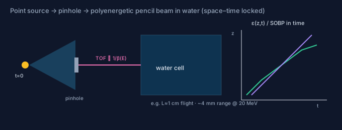
Computing \(\varepsilon(z,t)\) (or the dose rate) for a realistic \(\mathrm{d}N/\mathrm{d}E\) is the content of Exercise 11, Part B(a): every energy bin arrives at a different time and stops at a different depth; the SOBP is the cumulative integral over those contributions.
4. Where does the kinetic energy go?
Bethe–Bloch describes the mean energy lost by the projectile. Microscopically that energy is transferred to the medium mainly by ionizing and exciting water molecules: secondary electrons are liberated along the track. Those electrons scatter, slow down, and — in water — become trapped in a polarization cloud of surrounding \(\mathrm{H_2O}\) dipoles: the hydrated / solvated electron \(e_{\mathrm{aq}}^-\). Other radicals (\(\cdot\mathrm{OH}\), \(\cdot\mathrm{H}\), …) form on related radiolysis pathways (see Buxton et al., J. Phys. Chem. Ref. Data 17, 513 (1988)).
On longer timescales the deposited energy density \(\varepsilon(\mathbf{r},t)\) also appears as heat and pressure (stress / heat confinement → ionoacoustics in later lectures). For optical probing on sub-nanosecond to tens-of-nanoseconds scales, the decisive messenger is often the solvated electron: it absorbs strongly in the visible/NIR, so a probe laser sees a transient drop in transmission wherever energy was deposited.
5. Optical probe: we can see the solvated electron
A continuous-wave or pulsed probe through the water cell converts the depth–time map of energy deposition into a transmission image \(T\approx e^{-\alpha}\) with absorbance \(\alpha=\beta\,c\,l\) set by the solvated-electron concentration \(c\) (Beer–Lambert). That is the bridge from “spectrum in vacuum” to “something you can watch with a camera” — and the starting point for chirped-pulse probing and interferometry in Lecture 12.
Bottom line. RCF stacks give the best integral SOBP snapshots. A laser-driven point source plus a pinhole gives a polyenergetic pencil beam whose SOBP is intrinsically time-resolved. The energy that builds that SOBP in water ends up — transiently — in species we can see, notably the solvated electron.