This sheet accompanies Lecture 11. Part A treats focused-proton bunch timing; Part B the time-resolved energy deposition and solvated-electron transmission in water.
Part A — Spatial and temporal characteristics of a focused proton bunch
Consider a CALA-like setup: a \(30\,\mathrm{fs}\) laser pulse generates a proton spray with energies up to \(20\,\mathrm{MeV}\). A quadrupole doublet captures the central spray and focuses a design energy of \(10\,\mathrm{MeV}\) onto a platform \(2\,\mathrm{m}\) away. About \(10^{6}\) protons reach a \(\sim 1\,\mathrm{mm}\) spot; the transported relative energy spread is \(\sim 5\%\).
- Estimate the mean penetration depth of the protons (e.g. NIST PSTAR, water or tissue-equivalent).
- Estimate the variance of the range due to (i) range straggling and (ii) the initial energy spread. Which contribution dominates?
- Estimate the duration of the proton bunch at impact (TOF difference across the energy band).
- Estimate the trajectory / slowing-down time of the mean-energy proton while it stops. Conclude whether the deposition can be treated as instantaneous for µs-scale acoustics.
Part B — Time-resolved deposition and transmission in water
LION / CALA pump–probe context (Prasselsperger+): protons from a thin foil / water leaf with a typical spectrum extending to \(20\,\mathrm{MeV}\) and amplitude of order \[ \frac{\mathrm{d}^2 N}{\mathrm{d}E_{\mathrm{kin}}\,\mathrm{d}\Omega} \approx 10^{6}\,\frac{\text{protons}}{1\%\,E_{\mathrm{kin}}\cdot\mathrm{msr}} \] (cf. ALPA proton database). A water cell sits \(L=1.7\,\mathrm{cm}\) behind the target; a square aperture of side \(d=500\,\mu\mathrm{m}\) selects a pencil beam (aperture ≪ beam size at that distance). Assume all protons are born at \(t=0\).
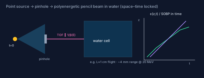
- Deposited power density \(\pi(z,t)\). Calculate the deposited power density as a function of depth \(z\) into the sample and time \(t\). Use Bethe–Bloch / range–energy relations from Exercise 10 and weight by the spectrum through the aperture. (Equivalently: construct the cumulative energy density \(\varepsilon(z,t)=\int_{-\infty}^{t}\pi(z,t')\,\mathrm{d}t'\).)
- Transmission image. Convert the two-dimensional energy-density map into a transmission image by assuming that the solvated electron dominates absorption (Beer–Lambert; \(T=\mathrm{e}^{-\alpha}\), \(\alpha=\beta\,c\,l\)). State clearly which lifetime / yield assumptions you make.
Tip: Part A shows that stopping is ≪ ns; Part B asks for the structured \(\varepsilon(z,t)\) that optical probes can see via \(e_{\mathrm{aq}}^-\) (Lecture 11 §4–5).