- Lecture 11 left us with a prediction: deposited energy darkens water via solvated electrons. Today we ask how to probe that — and what remains after the water brightens again.
- Chirped-pulse probing (CPP) maps wavelength to time in one shot and recovers a near-\(\pi(z,t)\) map of energy deposition (Prasselsperger et al., PRL 2021 — results shown in class slides).
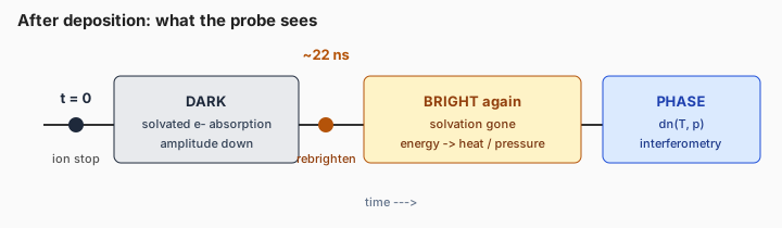
- Heavy-ion water experiments (GSI) show the same darkening; after \(\sim 22\,\mathrm{ns}\) the water is bright again — solvation is gone. The energy is then heat and pressure.
- Little amplitude modulation remains, but phase modulation does: Shadowgraphy, Schlieren, and especially Interferometry. Candle demo → Exercise 12. Closing: Mo Bragg curve visible in the interferogram at kGy / few-K heating.
- Transmission change — dissolve salt / sugar in water (amplitude object).
- Candle / flame with imaging lens — phase object nearly invisible when focused.
- Schlieren (knife edge) and defocused shadowgraphy — \(\propto\nabla n\) vs. \(\propto\nabla^2 n\).
- Mach–Zehnder with candle — fringes encode phase; block reference arm → absorption image.
Lecture 11 constructed a time-resolved SOBP and argued that solvated electrons make the deposition optically dark. We do not yet discuss “water becomes bright again” as a radiolysis puzzle — we simply take the experimental fact that darkness is transient, and focus on the probe methods.
1. Chirped-pulse probing
A continuous-wave probe integrates over the whole history. A short probe pulse freezes one instant — but scanning delay costs many shots. Chirped-pulse probing stretches a broadband pulse (glass block or fibre) so that different colours arrive at different times. The key experimental trick is an imaging spectrometer: image the water cell from the side onto the spectrometer slit — the slit coordinate is then depth \(z\) into the sample (where the Bragg / SOBP structure lives). The grating disperses wavelength perpendicular to the slit, so the camera’s other axis is \(\lambda\). With a chirped probe, \(\lambda\leftrightarrow t\), and one frame is the 2D transmission map \(T(z,t)\).
In the LION / CALA probe path the chirp is often “for free”: a \(\sim 60\,\mathrm{m}\) fibre from the oscillator already stretches a \(\sim 15\,\mathrm{fs}\) pulse into the picosecond–nanosecond regime (estimate this stretch in Exercise 12, Part B).
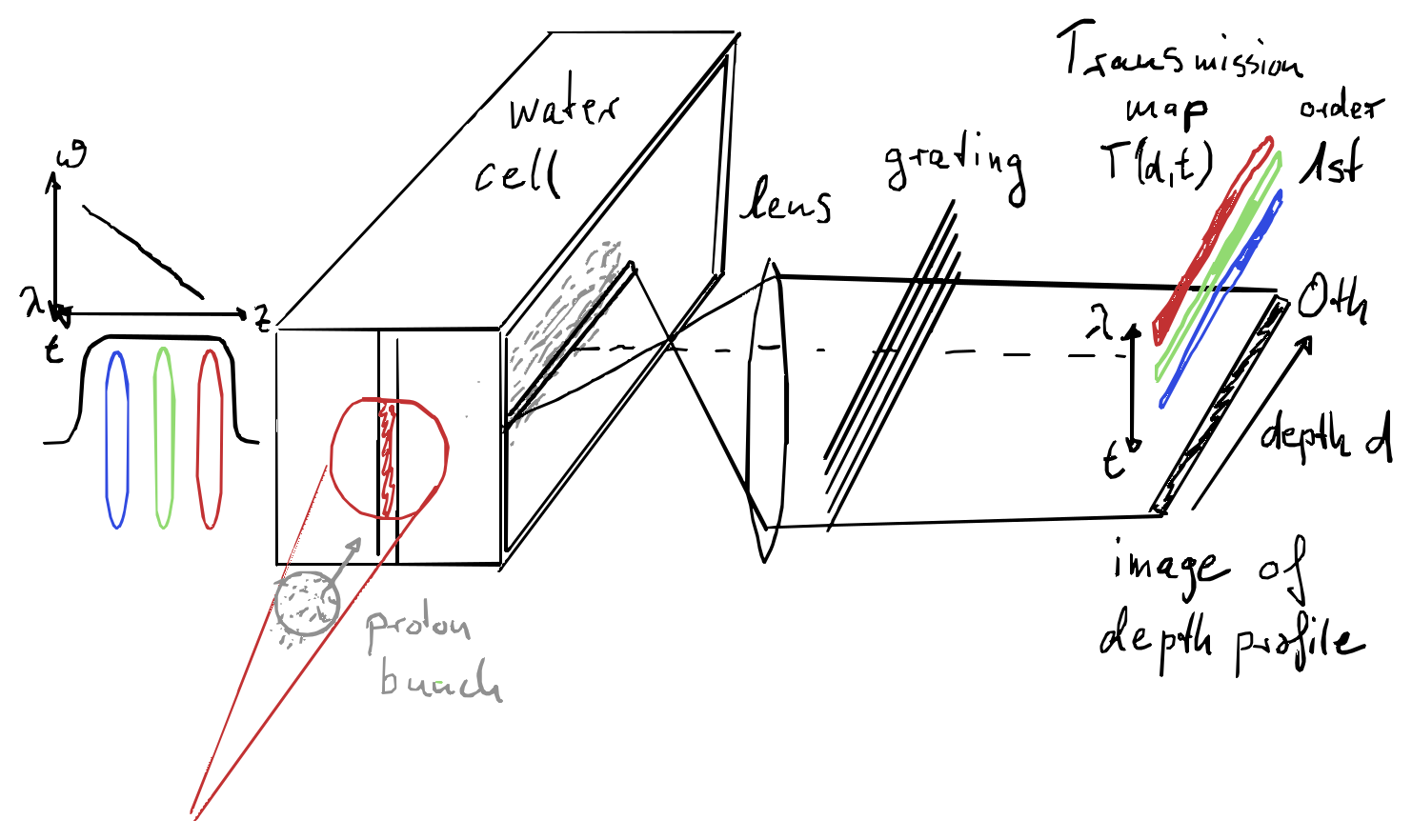
With laser-driven protons into water this yields a single-shot map close to the deposited power density \(\pi(z,t)\) discussed in Exercise 11 — see Prasselsperger et al., Phys. Rev. Lett. 127, 186001 (2021). Representative data frames are shown in the accompanying lecture slides (not reproduced here). Solvation itself takes tens of picoseconds after proton impact; the optical signature then tracks the local energy deposition in space and time.
2. Darkening with heavy ions; \(\sim 22\,\mathrm{ns}\) lifetime
Complementary measurements with conventional heavy-ion bunches in water (GSI / SIS-18; Mo / U beams, optical probe synchronised to the bunch; work of Liese, Prasselsperger and collaborators) also show a clear transmission drop that follows the Bragg region while the bunch is present. The underlying absorber is again consistent with the solvated electron.
Across laser-proton and heavy-ion campaigns the empirical wrap-up is sharp: after roughly \(22\,\mathrm{ns}\) the water is bright again — the solvated-electron population has disappeared. Amplitude modulation of a probe laser is then essentially gone.
3. Where is the energy then — and can we still see something?
The kinetic energy of the ions has been transferred to the medium: ionization, excitation, secondary electrons, then thermalization of the electronic system with the molecular bath. After the transient optical absorbers recombine, that energy lives on as temperature and pressure. A temperature (or density) change shifts the refractive index \(n(T,p)\). A probe wave therefore picks up a phase shift \[ \Delta\varphi = \frac{2\pi}{\lambda}\int \Delta n\,\mathrm{d}l \] even when its amplitude is barely changed. Heat confinement and stress confinement (Lecture 14) decide how long that \(\Delta n\) persists and whether a pressure wave radiates away.
4. Making phase visible: Shadowgraphy, Schlieren, Interferometry
A pure phase object is invisible in perfect imaging (Demo: candle flame with a well-focused imaging lens — almost nothing). Three classical remedies:
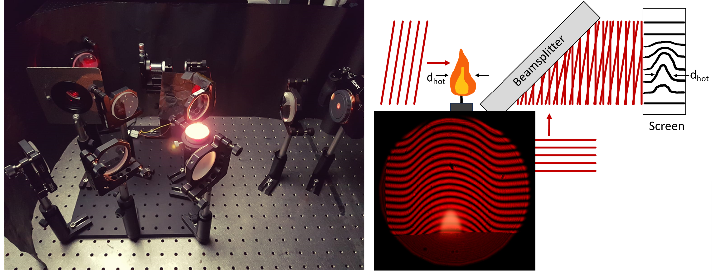
On the detector the intensity is the two-beam interference
\[
I \propto |E_{\mathrm{r}}+E_{\mathrm{o}}|^2
= |E_{\mathrm{r}}|^2+|E_{\mathrm{o}}|^2
+ 2\,\mathrm{Re}\!\left(E_{\mathrm{r}}^* E_{\mathrm{o}}\right).
\]
With a small angular carrier between the arms the cross term is a fringe pattern. A Fourier-sideband filter
recovers the complex object wave (amplitude and phase); a reference interferogram without the object
removes residual fringe curvature
(Exercise 12; helper script e09_interferometry.m).
5. Closing experiment: Bragg curve in the interferogram
With monoenergetic heavy ions (e.g. \(^{100}\mathrm{Mo}\) at \(\sim 300\,\mathrm{MeV/u}\), \(\sim 8\times 10^{8}\) ions, \(\sim 3\,\mathrm{mm}\) spot, dose \(\sim\mathrm{kGy}\) at the Bragg peak, local \(\Delta T\sim\) a few kelvin) the fringe shift in water literally sketches the Bragg curve. Transient features — outgoing sound waves — appear because the energy is deposited in a short bunch. These GSI runs used conventional monoenergetic bunches: a clean Bragg peak, and therefore a well-localised source of the acoustic wave at the peak. That is the optical motivation for ionoacoustics / I-BEAT — but to do the same with laser-driven protons we first need an energy-selecting beamline.
Bridge to Lectures 13–14. Optical phase shows heat and pressure after \(\sim 22\,\mathrm{ns}\). Acoustic tracing of the Bragg peak (I-BEAT) wants a monoenergetic, focused pencil beam — hence quadrupole transport next (Lecture 13), then the thermoacoustic wave equation (Lecture 14).