This sheet accompanies Lecture 12. Part A: candle temperature from interferograms. Part B: fibre chirp of the optical probe — the same dispersion that enables chirped-pulse probing.
Part A — Candle interferometry
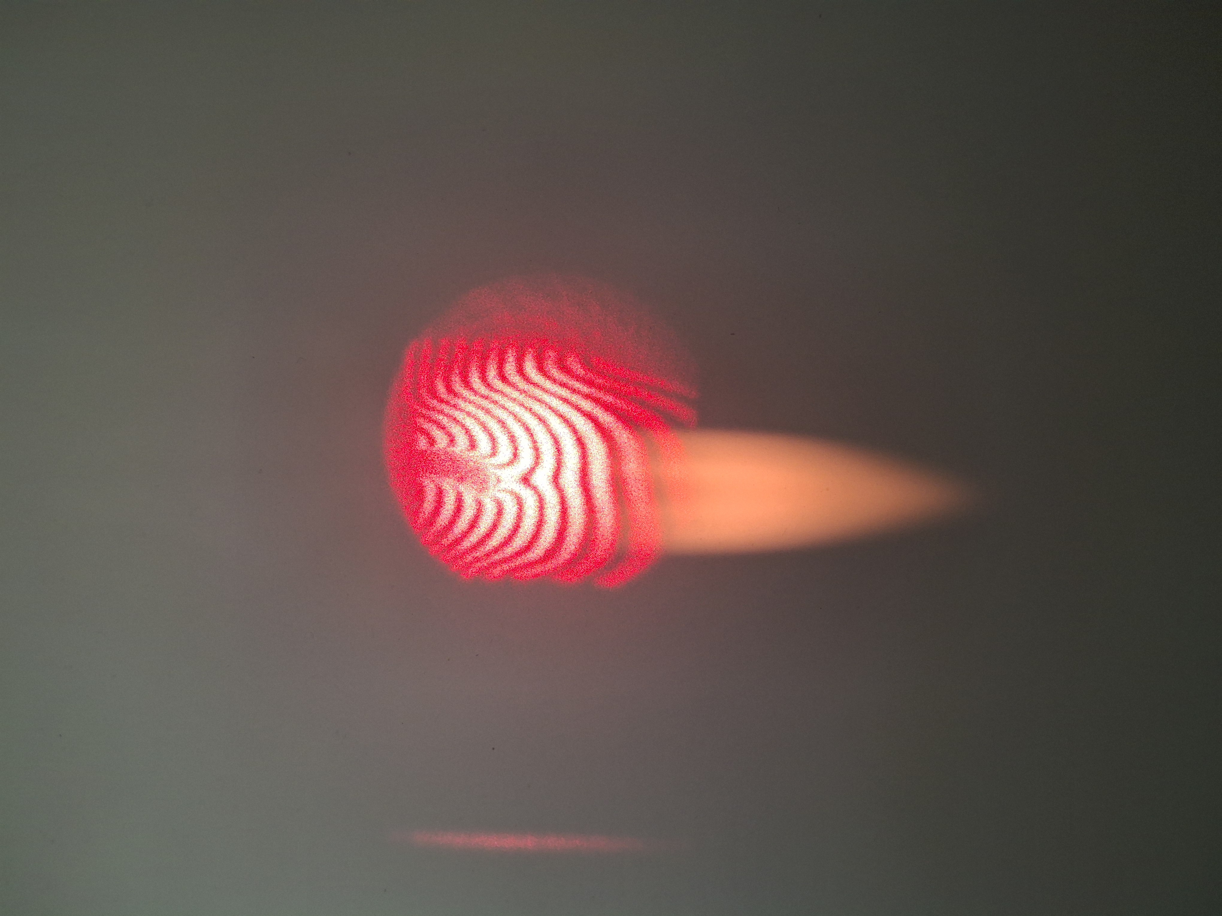
exercise12_candle_int.jpg).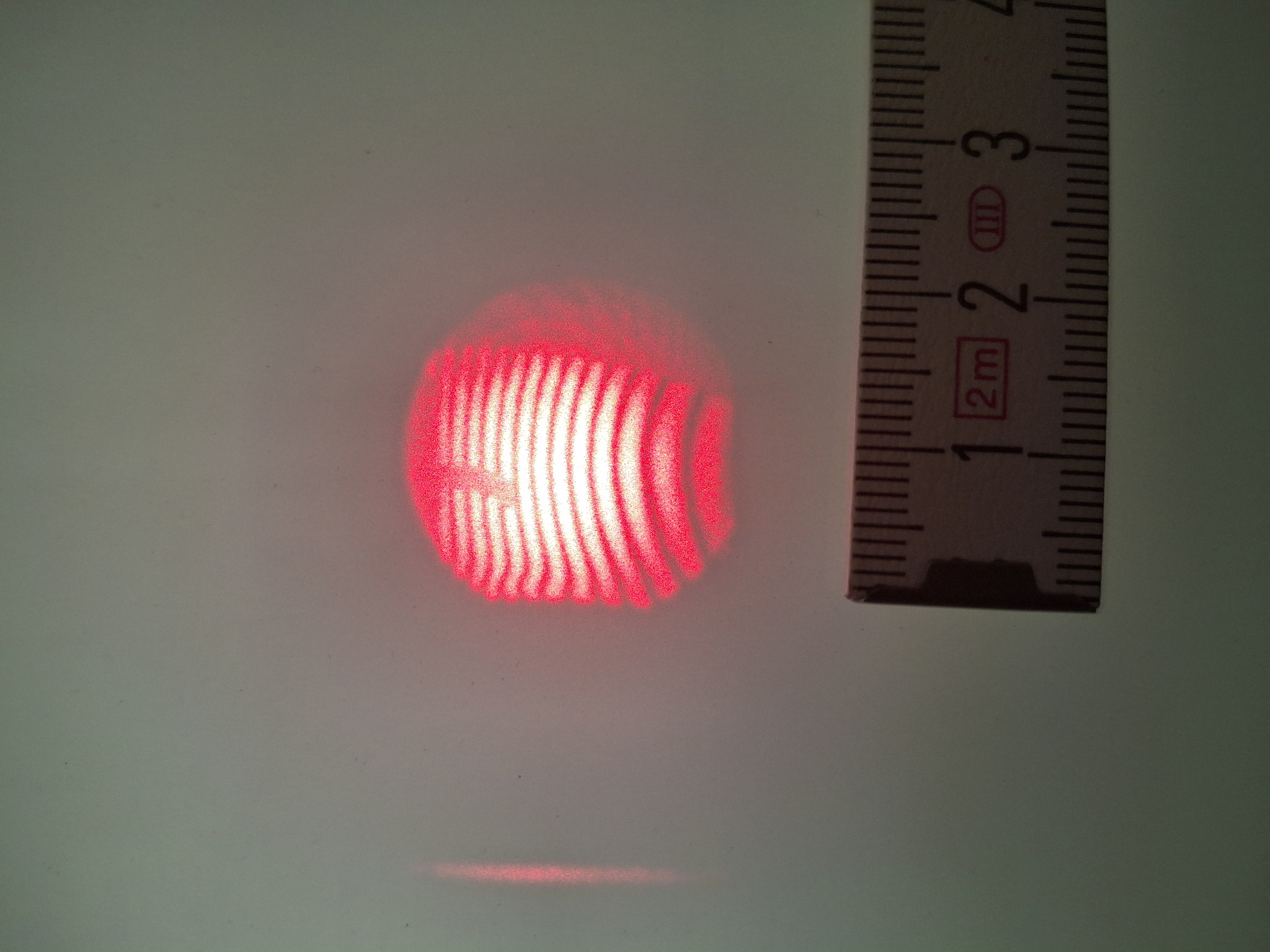
exercise12_candle_ref.jpg).- Using the interferometric images above, describe a method for obtaining a rough estimate of the candle temperature. Discuss the resulting estimate, the choice of readout position, and any potentially unphysical results. What issues arise with this method?
- Suggest (or identify) an approach to determine the temperature distribution — either as a full map or as a lineout at a fixed height. You may focus on the lineout if a full map is impractical.
-
(Optional / coding.)
Recover the complex object wave via Fourier sideband filtering (Lecture 12). Divide by the reference
object wave, unwrap the phase, and fit a simple radial temperature model
(e.g. Gaussian \(T(r)\)). A MATLAB starter is provided as
e09_interferometry.m(expects the jpg filenames; rename or edit paths as needed).
Air: \(n-1 \propto\) density; ideal gas \(\Rightarrow n-1\propto 1/T\). Fringe shift \(\Delta\varphi = (2\pi/\lambda)\int\Delta n\,\mathrm{d}l\). A crude cylinder estimate uses the half-fringe radius (see Lecture 12). Abel inversion or a forward Gaussian fit is more stable than a single-number estimate.
Part B — Fibre chirp of the probe
In the LION pump–probe setup the probe is taken from the femtosecond oscillator (assume transform-limited Gaussian pulses with intensity FWHM \(\tau_0 = 15\,\mathrm{fs}\)) and guided to the experiment through a fibre of length \(L\sim 60\,\mathrm{m}\). Dispersion stretches the pulse — that stretch is the chirp exploited in Lecture 12.
- Estimate the probe pulse duration after \(\sim 60\,\mathrm{m}\) of fibre. Use the Gaussian / GDD relation from the lecture or standard ultrashort-pulse texts, e.g. \[ \tau = \tau_0 \sqrt{1+\left(\frac{4\ln 2\,|\phi_2|}{\tau_0^2}\right)^2}, \qquad \phi_2 = \beta_2 L, \] with group-velocity dispersion \(\beta_2\) of the fibre (fused silica / SMF near \(800\,\mathrm{nm}\): look up a value, or take \(\beta_2\sim +40\,\mathrm{fs}^2/\mathrm{mm}\) as a crude glass estimate unless a better number is given in class). State your \(\beta_2\) and the resulting \(\tau\).
- In one sentence: why is this lengthening useful for chirped-pulse probing of the \(\sim\mathrm{ns}\) solvated-electron dynamics, rather than a problem to be recompressed away?