1. Gaussian and not so Gaussian pulses
We mainly treat laser pulses as if they were perfectly Gaussian. This is convenient both in space and in time: the Gaussian beam is the fundamental solution of the paraxial wave equation (which itself is an approximation to the Helmholtz equation), and the Gaussian temporal envelope is the simplest model for a transform‑limited pulse. Also, the Fourier-transform of a Gaussian is a Gaussian.
In reality, however, real laser pulses are rarely perfectly Gaussian. Both the temporal profile and the spatial intensity distribution can deviate significantly from a Gaussian. This has important consequences:
- Finite temporal contrast: In addition to the main pulse there is pre-pulse and pedestal light at lower intensity that arrives long before the peak. Because the peak intensity we are interested in is extremely high, even this weak early light is crucial: it defines the moment when the first plasma is created and the dynamics start. If you remove just one electron from each atom in a solid object – say, a table – you have already turned it into a plasma, and the table will disintegrate rather quickly.
- Spatial hot spots, side lobes, pedestal from scatter: the focal spot may have structure that drives ionization or plasma formation at different locations than a simple Gaussian model would suggest. This might not seem too relevant at first sight, but is so if you try to calculate the peak intensity in a given experiment correctly. It can also affect regions far off the central focus that one would not consider (i.e. you sometimes find damage in unexpected places and components).
As the peak intensities we are aiming at correspond to electric fields well above typical atomic binding fields, such non‑ideal features become crucial: even a small pre‑pulse can ionize the target before the main pulse arrives. Therefore, we must first understand how atoms are ionized by intense laser fields.
2. Strong-field ionization of atoms
We consider a simple one‑dimensional model of an atom, for instance hydrogen with ionization potential \( I_p = 13.6\ \mathrm{eV} \). The unperturbed atomic potential supports bound states up to the ionization threshold. When a laser field with insufficient photon energy for photo excitation (ionisation) is applied, ionization can occur nevertheless via two limiting mechanisms:
- Multi‑photon ionization (MPI),
- Field (tunneling) ionization (FI).
The relative importance of these processes is described by the Keldysh parameter, which we will introduce below.
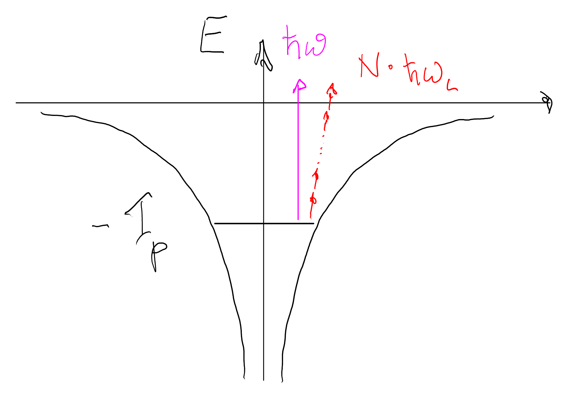
2.1 Multi‑photon ionization (MPI)
If the laser frequency \( \omega \) is such that a single photon carries much less energy than the ionization potential \( I_p \), i.e. \( \hbar\omega \ll I_p \), the atom can still be ionized by absorbing several photons simultaneously.
The minimum number of photons required is \[ N = \left\lceil \frac{I_p}{\hbar\omega} \right\rceil . \] After absorbing \( N \) photons, the electron can leave the atom with kinetic energy \[ E_{\text{kin}} = N \hbar\omega - I_p . \]
In perturbation theory, the N-photon transition amplitude is proportional to the N-th power of the electric field, \(\mathcal{A}_N \propto E^N\). Since the intensity scales as \(I \propto E^2\), the corresponding transition probability (or rate) scales like
\[ W_N \propto |\mathcal{A}_N|^2 \propto E^{2N} \propto I^N. \]
Multi-photon ionization is therefore strongly suppressed at low intensities and only becomes significant once the laser field substantially perturbs the bound-electron motion. In classical terms, the electron’s oscillation in the binding potential ceases to be perfectly harmonic.
2.2 Field ionization / tunneling ionization (FI)
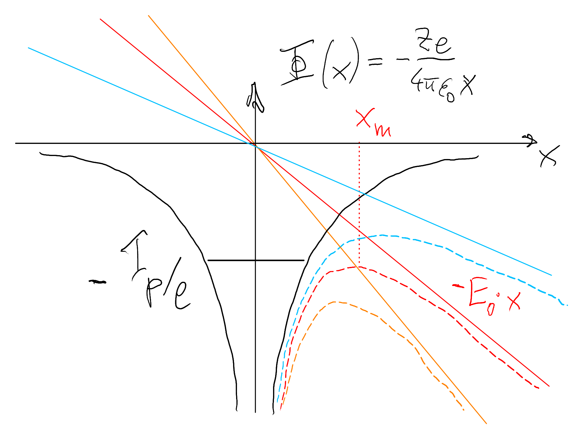
In the opposite limit of very strong fields and not too high frequency, the laser field can be viewed as quasi‑static during one optical cycle. The electric field then tilts the atomic potential, forming a barrier through which the electron can tunnel, as sketched in Figure 4.2. This is called field ionization or tunneling ionization.
As an order-of-magnitude estimate, we can compute a “threshold field” \(E_{\text{th}}\) at which the atomic binding barrier is essentially suppressed by the external field. For simplicity we consider hydrogen (\(Z=1\)) and write the combined potential energy of the electron (Coulomb + external field) as
\[ U(x) = -\frac{e^2}{4\pi\varepsilon_0 x} - e E_0 x . \]
In the presence of the static field \(E_0\), this potential has a maximum (a saddle point) at some position \(x_m\). We find it by solving \(\mathrm{d}U/\mathrm{d}x = 0\):
\[ \frac{\mathrm{d}U}{\mathrm{d}x} = \frac{e^2}{4\pi\varepsilon_0 x^2} - e E_0 = 0 \quad\Rightarrow\quad x_m = \sqrt{\frac{e}{4\pi\varepsilon_0 E_0}} . \]
Inserting this back into \(U(x)\) gives the potential energy at the barrier top, \(U_m = U(x_m)\). A straightforward algebraic simplification yields
\[ U_m = -2\sqrt{\frac{e^3 E_0}{4\pi\varepsilon_0}} . \]
Ionization becomes very efficient once this barrier top is at (or above) the bound-state energy, i.e. when \(|U_m| \approx I_p\). Setting \(|U_m| = I_p\) and solving for the field amplitude \(E_0\) gives
\[ I_p = 2\sqrt{\frac{e^3 E_{\text{th}}}{4\pi\varepsilon_0}} \quad\Rightarrow\quad I_p^2 = \frac{4 e^3 E_{\text{th}}}{4\pi\varepsilon_0} = \frac{e^3 E_{\text{th}}}{\pi\varepsilon_0}, \] and thus \[ E_{\text{th}} = \frac{\pi\varepsilon_0}{e^3}\, I_p^2 . \]
For hydrogen with \(I_p = 13.6\ \mathrm{eV}\) this gives a characteristic threshold field of about \[ E_{\text{th}} \approx 3\times 10^{10}\ \mathrm{V/m}. \] For comparison, a simple estimate of the “Bohr field” based on the ground-state binding energy and the Bohr radius \(a_0 \approx 0.5\times 10^{-10}\ \mathrm{m}\) is \[ E_{\text{Bohr}} \approx \frac{I_p}{e\,a_0} \approx 2.7\times 10^{11}\ \mathrm{V/m}, \] i.e. almost an order of magnitude larger. Thus tunneling (barrier-suppression) ionization already becomes efficient at fields well below the internal “atomic” field scale.
2.3 Keldysh parameter
The relative importance of MPI and tunneling ionization is captured by the Keldysh parameter \[ \Gamma = \frac{t_{tunnel}}{\pi/\omega} = \frac{\omega}{eE_0}\sqrt{2 m_e I_p} = \sqrt{\frac{I_p}{\langle E_{kin} \rangle}}, \] where \( E_0 \) is the peak electric field and \( \omega \) the laser frequency, \( \langle E_{kin} \rangle \) is the cycle average of the kinetic energy of a free electron oscillating in the laser field (We'll come back to this quantity a lot). The limiting cases are:
- \( \Gamma \gg 1 \): multi‑photon regime (perturbative MPI).
- \( \Gamma \ll 1 \): tunneling (field) ionization regime.
In many practical situations, especially at intermediate intensities and near‑infrared wavelengths, both mechanisms can contribute and one should use more complete models such as the Keldysh or ADK ionization rates.
Once the first electrons are liberated, they can be further accelerated in the laser field and in any accompanying quasi‑static fields. These hot electrons can in turn ionize other atoms via collisions (collisional ionization), leading to an avalanche and rapid plasma formation.
3. Motion of a free electron in an oscillating electric field
After ionization, the electron is essentially free and is driven by the laser field. In a linearly polarized plane wave we can write (in the non‑relativistic limit) \[ m_e \frac{dv}{dt} = -e E_0 \cos(\omega_0 t), \] where \( E_0 \) is the peak electric field amplitude. Integrating once (and choosing the constant of integration such that \( v(0)=0 \)) we obtain \[ v(t) = \frac{eE_0}{m_e\omega_0} \sin(\omega_0 t). \]
The instantaneous kinetic energy is \[ E_{\text{kin}}(t) = \tfrac{1}{2} m_e v^2(t) = \frac{e^2 E_0^2}{2 m_e \omega_0^2} \sin^2(\omega_0 t). \] The cycle‑averaged kinetic energy is the so‑called ponderomotive energy: \[ U_p = \langle E_{\text{kin}} \rangle = \frac{e^2 E_0^2}{4 m_e \omega_0^2}. \]
3.1 Intensity and the \( I\lambda^2 \) scaling
For a plane wave with linear polarization, the peak intensity is related to the electric field by \[ I_0 = \frac{1}{2}\,\varepsilon_0 c\,E_0^2. \] Using \( \lambda_0 = 2\pi c / \omega_0 \), we can express the ponderomotive energy in terms of intensity and wavelength: \[ U_p = \frac{e^2 E_0^2}{4 m_e \omega_0^2} = \frac{e^2}{2 m_e \varepsilon_0 c \omega_0^2}\,I_0 = \frac{e^2 \lambda_0^2}{8\pi^2 m_e \varepsilon_0 c^3}\,I_0. \] Thus \[ U_p \propto I_0 \lambda_0^2, \] i.e. the ponderomotive energy scales linearly with intensity and with the square of the wavelength.
A commonly used numerical form for electrons is \[ U_p[\mathrm{eV}] \approx 9.3\times 10^{-14}\, I_0\!\left[\frac{\mathrm{W}}{\mathrm{cm}^2}\right]\, \lambda_0^2[\mu\mathrm{m}^2]. \] This scaling is essential for estimating how “violent” the electron motion in a given laser field will be.
3.2 “Relativistic power unit”
It is useful to relate the ponderomotive energy to the electron rest energy \( m_e c^2 \). From the expression above we can write \[ U_p = m_e c^2 \left( \frac{I_0 \lambda_0^2}{2 \pi P_{\text{rel}}} \right), \] where we have introduced a characteristic power scale \[ P_{\text{rel}} = \frac{4\pi \varepsilon_0 m_e^2 c^5}{e^2} \approx 8.7 \ \mathrm{GW} \] for electrons. For protons the corresponding scale is larger by a factor \( (m_p/m_e)^2 \approx 3\times 10^6 \), i.e. \[ P_{\text{rel}}^{(p)} \sim 30 \ \mathrm{PW}. \]
One might interpret this result as follows: when \[ I_0 \lambda_0^2 \sim P_{\text{rel}}, \] the cycle‑averaged oscillatory energy of an electron approaches its rest energy \( m_e c^2 \). At this point a non‑relativistic description is no longer adequate.
Because typical laser wavelengths used for high‑field experiments are of order micrometers, it is common to express the electron dynamics in terms of the dimensionless amplitude (normalized vector potential) \[ a_0 = \frac{eE_0}{m_e c \omega_0} = \sqrt{\frac{2U_p}{m_e c^2}} \approx 0.85\, \sqrt{ \frac{I_0}{10^{18}\ \mathrm{W/cm}^2} }\, \lambda_0[\mu\mathrm{m}]. \] The regime \( a_0 \gtrsim 1 \) is usually referred to as the relativistic laser regime.
3.3 No net energy gain in a plane wave
Despite the large oscillatory energies that can be reached, it is important to remember a central result already encountered in Lecture 2: a free electron in a pure plane wave does not gain net energy over many cycles. The ponderomotive energy is an oscillatory energy, not a net acceleration. To obtain a net energy gain, some form of rectification is required, for example by spatial inhomogeneity (focused beams, plasma gradients, boundaries, etc.) or by additional fields.