Laser-Ion Acceleration – Lecture 6: Plasma refractive index, nonlinear optics, and PIC

Core message

Pickup from Lecture 5: the ratio \(n_e/n_c\) decides whether we pursue electron acceleration in underdense gas or ion acceleration at overdense surfaces.
The refractive index \(\eta\) depends on \(n_e\) and the effective electron mass; ionization, ponderomotive expulsion, and relativistic motion all change \(\eta(\mathbf{r},t)\) — the plasma is a nonlinear optical element.
The full problem is Maxwell + kinetics; no closed analytic solution exists in general. PIC (particle-in-cell) is the practical numerical approach.
We introduce the interactive 1D3V PIC tool here; Exercise 6 applies it to underdense and overdense cases.

In-class demos

Plasma frequency — microwave transmitters (9.4 GHz / 0.43 GHz) and fluorescent tubes.
Underdense discharge between tips (5 kV) + shadowgraphy — plasma deflects light without blocking it.
Skin length — thin gold foil / eclipse goggles: metals transmit when thickness \(\lesssim\delta\).

Lecture 5 introduced the cold-plasma refractive index and the underdense/overdense distinction. Today we deepen the plasma response — dispersion, skin depth, and the processes that make \(\eta\) spatially and temporally variable — then connect to the fully coupled Maxwell–kinetic problem and the PIC method used throughout the rest of the course.

1. Pickup: underdense vs overdense

Recall from Lecture 5 (no full re-derivation here): a collisionless electron fluid has dielectric function \(\varepsilon(\omega) = 1 - \omega_p^2/\omega^2\) with plasma frequency \(\omega_p = \sqrt{n_e e^2/(\varepsilon_0 m_e)}\), refractive index \(\eta = \sqrt{\varepsilon}\), and critical density \(n_c = \varepsilon_0 m_e \omega^2/e^2\) defined by \(\omega_p = \omega\). For Ti:sapphire (\(\lambda_0 \approx 800\,\mathrm{nm}\)), \(n_c \approx 1.7\times 10^{21}\,\mathrm{cm}^{-3}\).

A plane electromagnetic wave in a cold plasma obeys the dispersion relation \[ \omega^2 = \omega_p^2 + c^2 k^2, \] from which the phase and group velocities follow: \[ v_\varphi = \frac{\omega}{k} = \frac{c}{\sqrt{1-\omega_p^2/\omega^2}}, \qquad v_g = \frac{\partial\omega}{\partial k} = c\sqrt{1-\omega_p^2/\omega^2}. \] Note \(v_\varphi v_g = c^2\): phase velocity can exceed \(c\), but energy and information travel with \(v_g < c\) in an underdense plasma.

For overdense plasmas (\(n_e > n_c\), \(\omega_p > \omega\)), the refractive index is imaginary and the field is evanescent with skin depth \[ \delta = \frac{c}{\sqrt{\omega_p^2 - \omega^2}} \;\approx\; \frac{c}{\omega_p} \quad (\omega_p \gg \omega). \] Interaction is confined to a layer of order \(\delta \sim \lambda_p/(2\pi)\).

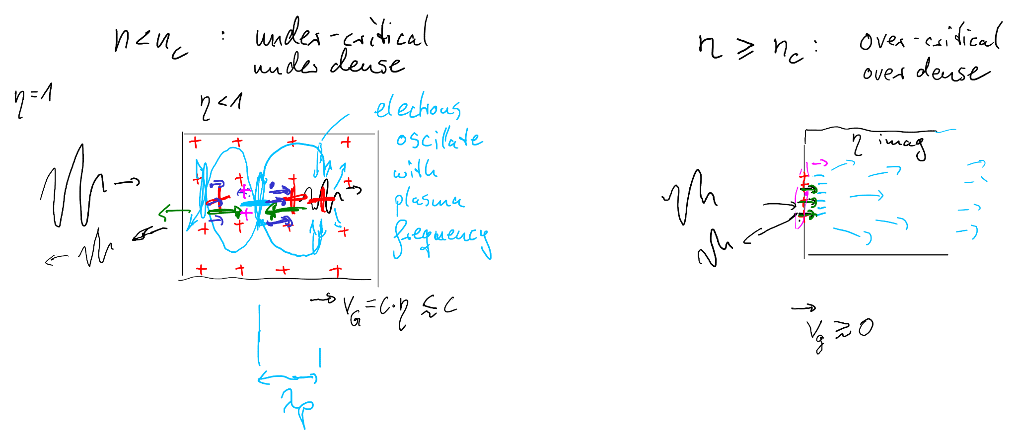
Pulse propagating with group velocity in underdense plasma. — Figure 6.1: Schematic of pulse propagation in an underdense plasma. The envelope and plasma wake structures move with the group velocity \(v_g < c\).

Two major directions in this course (recall the underdense/overdense sketch in Lecture 5):
• Underdense (\(n_e < n_c\)): laser propagates with \(v_g < c\) → electron acceleration in gas targets.
• Overdense (\(n_e > n_c\)): evanescent field, skin-depth interaction → ion acceleration from solid or liquid targets.

2. What changes the refractive index

Lecture 5 already noted that \(\eta(\mathbf{r},t)\) is not fixed. Three processes dominate at high intensity:

Relativistic motion: replace \(m_e \to \gamma m_e\) in the plasma response. The effective plasma frequency drops as \(\omega_p \propto 1/\sqrt{\gamma}\), and the critical density increases: \[ n_{c,\mathrm{rel}} \approx \gamma\, n_c. \] An overdense target can become relativistically transparent when \(a_0 \gtrsim 1\).
Ionization: raises \(n_e(\mathbf{r},t)\) during the pulse rise → local decrease of \(\eta\) → defocusing in underdense media; if \(n_e\) crosses \(n_c\), a plasma mirror forms.
Ponderomotive expulsion: electrons are pushed out of high-intensity regions → lower \(n_e\) on axis → higher \(\eta\) on axis → potential self-focusing.

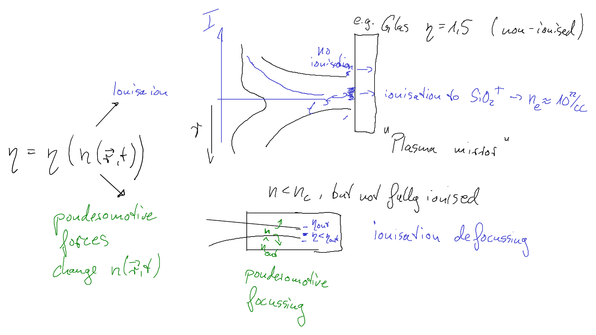
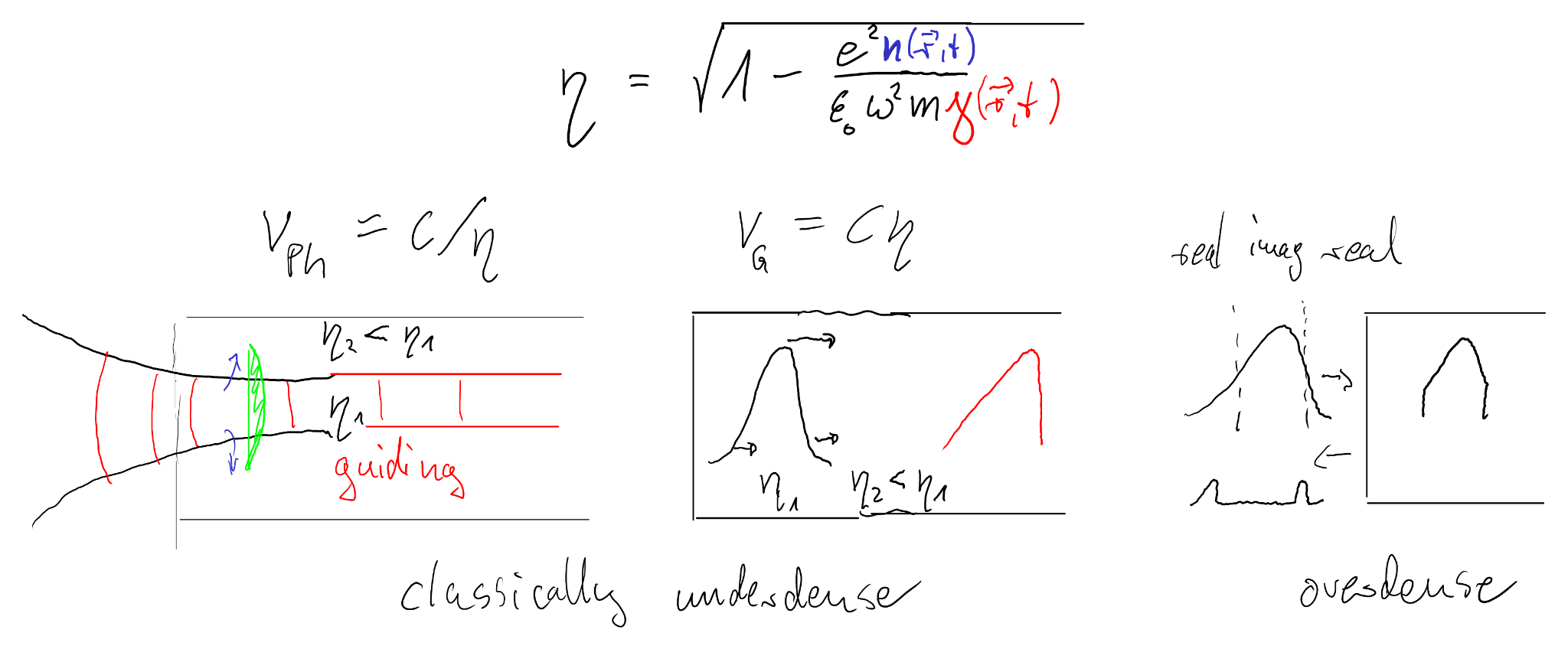
Ionization and ponderomotive effects changing refractive index. — Figure 6.2: Processes that modify \(n_e\) and/or the effective refractive index: ionization (defocusing / plasma mirror) and ponderomotive expulsion (self-focusing).

Relativistic plasma optics: self-focusing, steepening, induced transparency. — Figure 6.3: Relativistic plasma optics (schematic). From left to right: (i) relativistic self-focusing and channel guiding via intensity-dependent \(\eta\), (ii) pulse-front steepening / self-phase modulation as \(n(\mathbf{r},t)\) varies, (iii) relativistic induced transparency (“gate”) when \(\gamma\) raises the effective critical density so a previously overdense layer transmits.

These effects feed back on the fields: \(\eta(\mathbf{r},t)\) depends on how electrons move in the laser field, while the field is determined by Maxwell’s equations in the medium defined by \(\eta\). The fully coupled problem is not fully analytic — useful limits (uniform cold plasma, fixed \(n_e\), slowly varying envelope) guide intuition, but simulation is needed for realistic dynamics.

3. The complete problem → PIC

The full collisionless laser–plasma interaction problem couples Maxwell’s equations to a kinetic equation for each species \(s\) (electrons, ions) — typically the Vlasov equation. The distribution function \(f_s(\mathbf{x},\mathbf{p},t)\) evolves self-consistently with \(\mathbf{E},\mathbf{B}\).

Maxwell equations (SI units)

\[ \nabla \cdot \mathbf{E} = \frac{\rho}{\varepsilon_0},\qquad \nabla \cdot \mathbf{B} = 0, \] \[ \nabla \times \mathbf{E} = -\frac{\partial \mathbf{B}}{\partial t},\qquad \nabla \times \mathbf{B} = \mu_0 \mathbf{J} + \mu_0 \varepsilon_0 \frac{\partial \mathbf{E}}{\partial t}. \] Here \(\rho(\mathbf{x},t)=\sum_s q_s \int f_s\, d^3p\) and \(\mathbf{J}(\mathbf{x},t)=\sum_s q_s \int \mathbf{v}\, f_s\, d^3p\).

Vlasov equation

\[ \frac{\partial f_s}{\partial t} + \mathbf{v}\cdot\nabla_{\mathbf{x}} f_s + q_s \left( \mathbf{E} + \mathbf{v}\times\mathbf{B} \right)\cdot\nabla_{\mathbf{p}} f_s = 0, \] with relativistically consistent \(\mathbf{p}=\gamma m_s \mathbf{v}\), \(\gamma=\sqrt{1+(p/m_sc)^2}\).

Fluid models are obtained by taking velocity moments and adding closure assumptions. PIC (particle-in-cell) avoids such closures by evolving representative phase-space samples (“macro-particles”) directly, coupled to a grid-based Maxwell solver.

One PIC time step

Deposit charge density \(\rho^n\) and/or current \(\mathbf{J}^{n+1/2}\) from particles to the grid.
Field solve Maxwell’s equations on the grid (e.g. Yee/FDTD) → \(\mathbf{E}^{n+1}\), \(\mathbf{B}^{n+1/2}\).
Interpolate \(\mathbf{E},\mathbf{B}\) from grid nodes to each particle position.
Push particles with the Lorentz force (commonly the Boris pusher).
Apply boundary conditions (fields and particles), then repeat.

1D3V: one space dimension, three velocity components

In this course we use a 1D3V model: one spatial coordinate \(z\), but three velocity (or momentum) components \((v_x,v_y,v_z)\). All fields vary only with \(z\) and \(t\). The laser propagates along \(z\); transverse fields \((E_x,E_y,B_x,B_y)\) are evolved on the grid. The longitudinal field \(E_z\) is updated from the \(z\)-component of Ampère–Maxwell’s law, \[ \frac{\partial E_z}{\partial t} = -\frac{1}{\varepsilon_0}\,J_z, \] while Gauss’ law \(\partial E_z/\partial z = \rho/\varepsilon_0\) acts as a constraint preserved by charge-conserving current deposition.

Practical pitfalls (short list)

Courant condition: \(\Delta t \lesssim \Delta z / c\) for stable FDTD.
Resolve \(\omega_p\): \(\Delta t \ll \omega_p^{-1}\) in the densest region of interest.
Particle noise: statistical noise \(\propto 1/\sqrt{N_p}\); too few macro-particles per cell can hide real physics.
Boundary conditions: absorbing field boundaries (PML/damping), laser injection at \(z=0\), and appropriate particle boundaries.

4. Interactive PIC

The concepts above become tangible when you watch fields, densities, and phase space evolve in time. The interactive 1D3V PIC code below propagates the laser along \(z\) and lets you explore underdense propagation, near-critical slow-down, overdense reflection, wakefields, and relativistic transparency.

1D3V PIC tool: explore underdense and overdense regimes; vary \(n_e/n_c\), \(a_0\), pulse duration, and slab thickness. Monitor \(E_x\), \(E_z\), densities, and phase space. Guided cases with interpretation questions are in Exercise 6. Open fullscreen

5. Outlook

Lecture 7 treats collisionless absorption — how energy is transferred from the laser field to the plasma when the simple reflection/transmission picture is not enough. The PIC tool introduced here is the workhorse for exploring those mechanisms numerically.

Work through Exercise 6 before the tutorial: diagnostics, underdense dispersion and wakefields, overdense reflection and ion acceleration hints, and optional high-harmonic generation.

→ Exercise 6: PIC lab — underdense and overdense cases