This sheet accompanies Lecture 8: Crow/Mora sheath vs. test particle, Schreiber’s finite-radius model compared with Mora, and the optimal TNSA pulse duration. Hot-electron density \(n_{e,0}\) was already treated in Exercise 7, Part A.
Useful scripts in the course Exercises/ folder:
e04_plasmaexpansionCrowMora.m, e05_MoraVsSchreiber.m,
e05_SchreiberWithExp.m. Python is equally welcome.
1. Crow/Mora static sheath
- Fast electrons with density \(n_{e,0}\) exiting at a plasma–vacuum interface induce a positive surface charge. After a short transient, outgoing and returning fluxes balance: the electron density is in thermal equilibrium with the electrostatic potential, supported by a fixed step-like ion profile \(n_i=n_{i,0}\) for \(z<0\) and \(n_i=0\) for \(z\ge 0\). Formulate Poisson’s equation assuming Boltzmann hot electrons with average energy \(E_e(=k_B T_{e,h})\). Solve for the potential (tip: Crow et al. 1975; Mora 2003) and give \(E_s\) at the interface.
2. Mora expansion vs. test particle
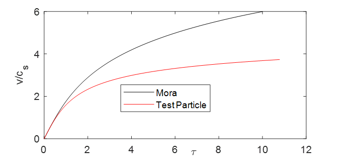
- Mora’s maximum ion velocity is \[ v_i \approx 2c_s\ln\!\bigl(\tau+\sqrt{1+\tau^2}\bigr)=2c_s\sinh^{-1}\tau, \] with \(c_s=\sqrt{q_i E_e/m_i}\) and \(\tau=\omega_{pi}t/\sqrt{2e}\). Compare this with the velocity a test ion of charge \(q_i e\) could gain in the fixed potential of Question 1. Produce a velocity–time plot (Mora vs. test particle), e.g. with the provided MATLAB script or your own code.
3. Approximating Schreiber and comparing to Mora
-
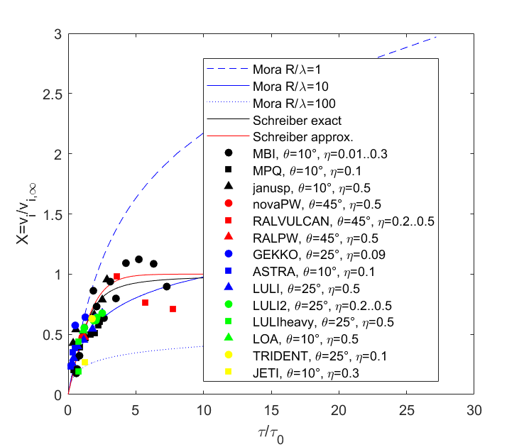
Schreiber’s finite-radius model reads
\[
\frac{\tau_L}{\tau_0}
= X\left(1+\frac12\frac{1}{1-X^2}\right)+\frac12\,\mathrm{atanh}\,X,
\]
where \(X=v_i/v_{i,\infty}\), \(\tau_0=R/v_{i,\infty}\), and
\(v_{i,\infty}=\sqrt{2ZE_\infty/m_i}\) with
\(E_\infty=(mc^2/2)\sqrt{2\eta P_L/P_R}\).
- Taylor-expand in \(X\) and obtain a simple approximate formula for \(v_i(\tau_L)\).
- Plot \(v_i/c_s\) vs. \(\tau\) for Mora and \(v_i/v_{i,\infty}\) vs. \(\tau_L/\tau_0\) for exact and approximate Schreiber. Relate the time scales via the hot-electron density (choose representative \(R/\lambda\), e.g. 100, 10, 1).
4. Optimal pulse duration in TNSA
- In the charged-disc / Schreiber picture the terminal ion energy scales with absorbed power, but acceleration lasts only for \(\sim\tau_L\). Using \[ \frac{\tau_L}{\tau_0} = X\left(1+\frac12\frac{1}{1-X^2}\right)+\frac12\,\tanh^{-1}X \] and \(v_{i,\infty}\propto\tau_L^{-1/4}\) at fixed energy \(E_L\), find the pulse duration \(\tau_{L,\mathrm{opt}}\) that maximises the ion energy. Evaluate for \(R=2\,\mu\mathrm{m}\) and absorbed energies \(\eta E_L=1\,\mathrm{J}\) and \(10\,\mathrm{J}\) (protons). Comment briefly on ATLAS-scale pulses (\(\sim 30\,\mathrm{fs}\), tens of joules).